Calculate Marginal Distribution: A Step-by-Step Guide

Introduction

Understanding how to calculate marginal distribution is crucial for professionals working with statistical data analysis, allowing them to evaluate the probabilities of various outcomes within a dataset. This concept is fundamental in the realm of statistics, particularly in the fields of probability and data interpretation. Calculations of marginal distribution help in analyzing the impact of single variables within multivariate datasets.

Marginal distribution calculations simplify the complexity of high-dimensional data by focusing on one variable at a time, making it easier to uncover underlying patterns and dependencies. Learning how to perform these calculations enhances data analysis skills and enables better decision-making.

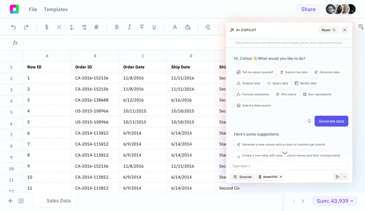
To facilitate this process, Sourcetable offers a powerful tool called an AI-powered spreadsheet assistant. This tool not only helps in calculating marginal distributions but also enhances overall productivity in managing data tasks. Discover how Sourcetable can streamline your statistical operations at app.sourcetable.com/signup.

How to Calculate Marginal Distribution

To calculate the marginal distribution effectively, understanding its components and the process is crucial. Marginal distribution, a core concept in statistics, offers insights into the probabilities of variables within a subset, irrespective of other variables.

Understanding Joint Distribution

Begin by identifying the joint probability mass function (p.m.f.) of the random variables involved. This is essential as the marginal distribution calculations are based on this distribution.

Calculating Marginal Distribution

For discrete variables, calculate the marginal distribution by summing the joint p.m.f. over all possible values of the other variables not being considered. For a variable X, the marginal p.m.f. is given by f_X(x) = P(X=x) = sum_y f(x, y). Conversely, for variable Y, it can be calculated using f_Y(y) = P(Y=y) = sum_x f(x, y). This method effectively reduces the dimensions of the data by focusing on one variable at a time.

Using the Marginal Distribution

Marginal distributions are not just theoretical constructs but have practical applications in risk assessment, machine learning, and even health care for evaluating treatment outcomes or disease prevalence.

Always ensure that your calculated marginal distributions satisfy the property of normalization, meaning that the probabilities add up to one, confirming the credibility of your distribution's results.

Visualizing and Analyzing Marginal Distribution

Once calculated, you can visualize the marginal distribution using histograms or other graphical representations to glean insights into the behavior of a single variable, thus simplifying complex multi-dimensional data for better analysis and decision-making.

Thoroughly summing the joint probabilities and understanding their implications allows for an accurate calculation and interpretation of marginal distributions essential in various statistical and analytical practices.

How to Calculate Marginal Distribution

Marginal distribution calculation offers a way to determine the probability distribution of a subset of random variables within a larger set. This process, known as marginalization, is essential for statistical analysis when one wants to focus on specific variables without considering others in the dataset.

Understanding Marginal Distribution

The marginal distribution of a random variable(s) gives the probabilities of various values of the variables independent of the other variables in a joint distribution. This distribution helps to understand the likelihood of single events or the probability of an event, assuming another has already occurred.

Calculating Marginal Distribution for Discrete Random Variables

To calculate the marginal probability mass function (p.m.f.) for a discrete random variable, sum the joint p.m.f. over all possible values of the other variable(s). For variable X, denoted as f_X(x), where x and y have a joint p.m.f. f(x, y), calculate f_X(x) by:

f_X(x) = \sum_y f(x, y).

Calculating Marginal Distribution for Continuous Random Variables

The process for continuous random variables involves integrating the joint probability distribution function over the range of the variable being omitted. For a variable X_i in a continuous set {X_1, X_2, ..., X_n}, the marginal distribution function f_{X_i}(x_i) is computed by:

f_{X_i}(x_i) = \int_{-\infty}^{\infty} \int_{-\infty}^{\infty} \ldots \int_{-\infty}^{\infty} f(x_1, x_2, ..., x_n) \, dx_1 \, dx_2 \ldots dx_{i-1} \, dx_{i+1} \ldots dx_n

Using Marginal Distribution in Statistical Analysis

Understanding how to calculate marginal distribution is crucial for analyzing the probability of events in statistical research, independent of other variables. It simplifies complex multivariable datasets to manageable, pertinent information relating to specific events of interest.

By mastering these calculations, statisticians can produce more targeted and meaningful inferential statistics and predictions, thereby enhancing the clarity and relevance of their analytical outcomes.

Examples of Calculating Marginal Distribution

Example 1: Two-Dimensional Discrete Variables

To calculate the marginal distribution of X from a joint probability distribution table of X and Y: Sum the probabilities across each row for X. Assume X can take values 1, 2, and Y can take values A, B with joint probabilities as follows. For X=1, Y=A (0.2); X=1, Y=B (0.1); X=2, Y=A (0.4); X=2, Y=B (0.3). The marginal distribution of X is: P(X=1) = 0.2 + 0.1 = 0.3 and P(X=2) = 0.4 + 0.3 = 0.7.

Example 2: Continuous Random Variables

For continuous variables X and Y where their joint probability density function (pdf) is given, integrate out Y to find the marginal pdf of X. If the joint pdf is f_{X,Y}(x,y) = e^{-(x+y)}, the marginal pdf of X is obtained by integrating Y over all possible values: f_X(x) = \int_{-\infty}^{\infty} e^{-(x+y)} dy. This integrates to f_X(x) = e^{-x}.

Example 3: Using Conditional Probabilities

To derive the marginal probability from conditional probabilities and the probability of the conditioning event, use the formula P(A) = P(A|B)P(B) + P(A|eg B)P(eg B). For instance, if the likelihood of rain (A) given that it is cloudy (B) is 0.5 and the probability of not raining given it is not cloudy (eg B) is 0.1, with the probability of it being cloudy or not being 0.3 and 0.7 respectively, then P(rain) = 0.5*0.3 + 0.1*0.7 = 0.22.

Example 4: Sum of Independent Random Variables

For independent random variables X and Y with known distributions, the marginal distribution of the sum Z=X+Y can be found by the convolution of their individual distributions. If X and Y are both uniformly distributed from 0 to 1, the probability density function of Z can be calculated using the convolution formula: f_Z(z) = \int_{-\infty}^{\infty} f_X(x) f_Y(z-x) dx.

Example 5: Multivariate Normal Distribution

In multivariate normal distributions, determining the marginal distributions of subsets of variables is straightforward. Given a joint normal distribution of X and Y with parameters μ_X, μ_Y, σ_X^2, σ_Y^2, ρ_XY, the marginal distribution of X alone is a normal distribution with mean μ_X and variance σ_X^2, independently of Y's values.

Master Calculations with Sourcetable

Intuitive AI Assistance for Every Calculation

Whether you're tackling complex statistical problems or simple arithmetic, Sourcetable is equipped to handle any mathematical challenge. Its AI-powered capabilities simplify computing tasks, transforming even the daunting process of how to calculate marginal distribution into an effortless task.

AI-Powered Spreadsheet for Optimal Learning

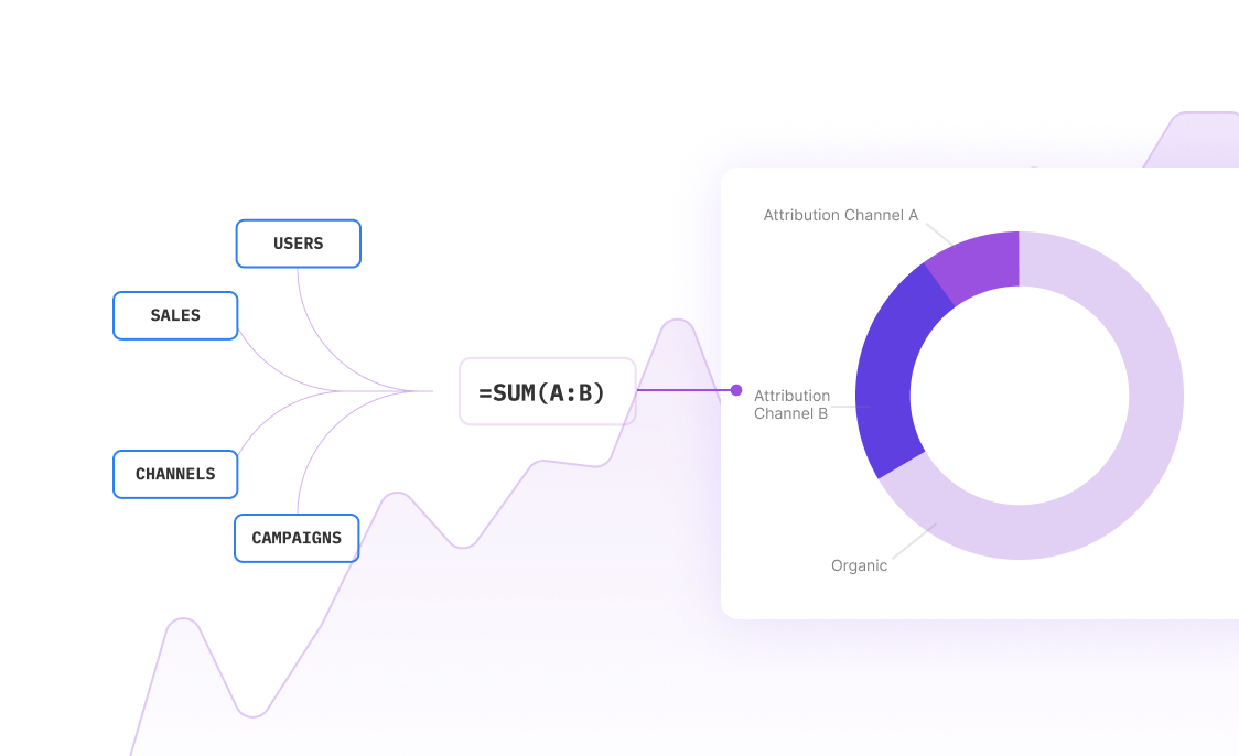
Sourcetable merges the power of artificial intelligence with the familiarity of spreadsheets. Pose a question, and the AI assistant not only performs calculations but also visualizes them directly within the spreadsheet interface. This feature is not just about getting answers but understanding the process.

Real-Time Explanations Enhance Understanding

For students and professionals alike, Sourcetable’s chat interface stands out by offering step-by-step explanations of how calculations are performed. When learning how to calculate marginal distribution, for example, it details each step in the chat, enhancing comprehension and retention of the concept.

Flexible and Versatile Tool for Diverse Needs

Sourcetable is designed for versatility. Whether you're studying for an exam, analyzing data for work, or simply exploring mathematical concepts, Sourcetable adapts to your needs, making it an indispensable tool for anyone looking to enhance their numeracy skills.

Conclusion

Understanding how to calculate marginal distribution is crucial for statistics and data analysis. By mastering this technique, you can extract relevant probabilities from joint probability distributions, fundamental in fields like economics, psychology, and machine learning.

Easy Calculation with Sourcetable

Sourcetable, an AI-powered spreadsheet, offers a streamlined solution to perform these important calculations. Its intuitive interface and powerful computational abilities make calculating marginal distribution more accessible, even for complex data sets.

Experiment with AI-generated data on Sourcetable to enhance your analytical skills and understand real-world applications. This hands-on experience is invaluable for learners and professionals alike.

Start optimizing your data analytics workflow today. Try Sourcetable for free at app.sourcetable.com/signup.