Calculate CDF from PDF

Introduction

Understanding the conversion from PDF (Probability Density Function) to CDF (Cumulative Distribution Function) is essential for anyone working with statistical data analysis or probability. This transformation plays a crucial role in interpreting data distributions and probabilities, allowing for deeper insights into statistical data. Calculating the CDF from a PDF involves integrating the probability density function from the lower bound to a specific value, thus indicating the probability of a variable falling within that range.

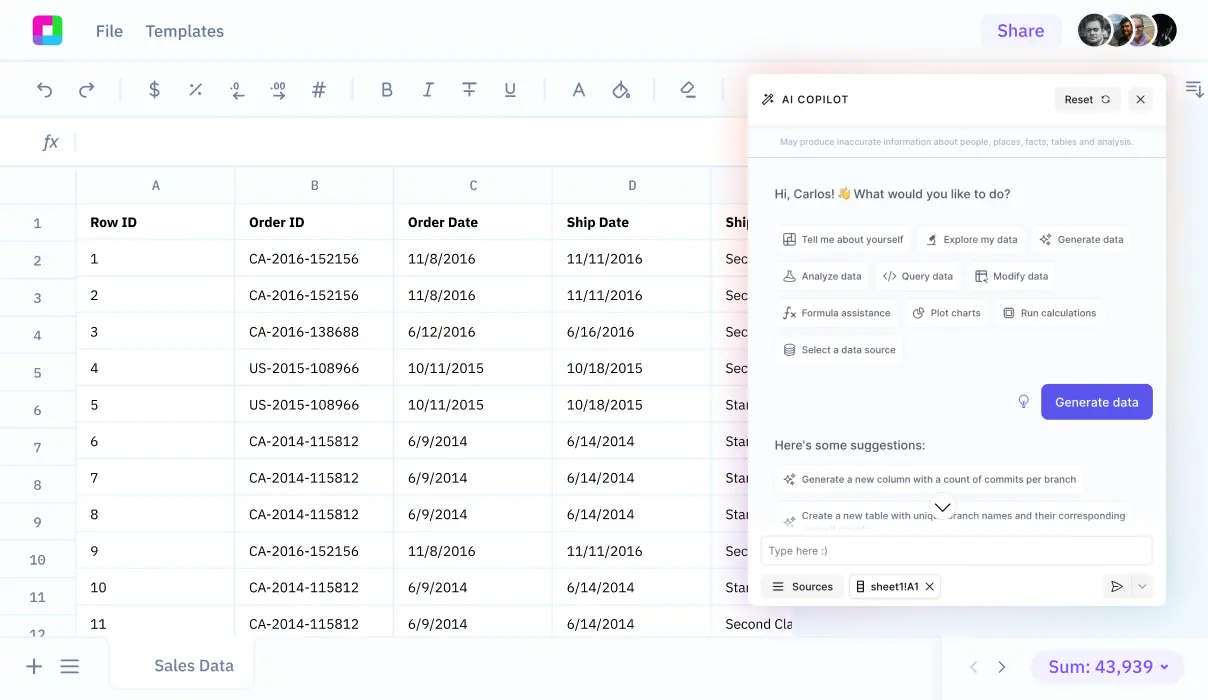
This article will guide you through the steps to calculate the CDF from a PDF with clarity and precision. Additionally, we will explore how Sourcetable lets you perform this calculation and more using its AI-powered spreadsheet assistant, which you can try at app.sourcetable.com/signup.

How to Calculate CDF from PDF

To calculate the Cumulative Distribution Function (CDF) from the Probability Density Function (PDF) for a continuous random variable, integrate the PDF. Use the formula F(x) = ∫[−∞,x] f(t) dt, where f represents the PDF and x the value up to which the probability is calculated. This process yields the CDF, F(x), which measures the probability that the random variable takes a value less than or equal to x.

Steps for Calculating CDF

Begin by identifying the PDF of the continuous random variable, represented as f(t). Proceed by integrating this function from negative infinity to x. This integral calculation quantifies the accumulated probability and thus, constructs the CDF, F(x).

Relationship Between CDF and PDF

The CDF F(x) can be derived by integrating the PDF f(t). Conversely, the PDF can be found by differentiating the CDF. This integral and differential relationship ensures that the PDF accurately represents the rate of change of probabilities detailed by the CDF.

Understanding and applying the integral process for CDF calculation is crucial for accurately analyzing the distribution and probabilities of continuous random variables.

How to Calculate CDF from PDF

Understanding how to calculate the Cumulative Distribution Function (CDF) from the Probability Density Function (PDF) is essential for statistical analysis involving continuous random variables. This section provides a concise guide on performing this calculation efficiently.

Step-by-Step Guide

To derive the CDF from a given PDF, one needs to integrate the PDF over the desired range. The formula to calculate the CDF, denoted as F(x), from the PDF, denoted as f(x), is given by F(x) = \int_{-\infty}^x f(t) \, dt. This fundamental relationship underscores that the CDF at any point x represents the area under the PDF curve from -∞ to x.

Normalization Condition

For the calculation to be valid, the total area under the PDF must equal one. This condition ensures that the PDF correctly represents the probability distribution of a random variable.

Example Application

Consider a scenario where a random variable X represents the time, in minutes, a person waits for an elevator. The maximum wait time is 2 minutes. The PDF in this case might be defined as follows:f(x) = 0 for x < 0, f(x) = x for 0 \leq x \leq 1, f(x) = 2-x for 1 < x \leq 2, and f(x) = 0 otherwise. To find, for example, F(0.5), compute F(0.5) = \int_{0}^{0.5} t \, dt = 0.125, and similarly, F(1.5) can be computed by F(1.5) = \int_0^1 t \, dt + \int_1^{1.5} (2-t) \, dt = 0.875.

Deriving PDF from CDF

If necessary, the original PDF can be retrieved by differentiating the CDF. This operation confirms that the PDF and CDF are fundamental inverses in distribution function calculations.

This concise explanation provides clear guidelines on how to compute the CDF from the PDF for any continuous random variable, reinforcing fundamental probabilistic concepts in practical applications.

Calculating CDF from PDF: Practical Examples

Example 1: Uniform Distribution

Consider a uniform distribution with a PDF defined as f(x) = 1 for 0 \leq x \leq 1. To find the CDF, integrate the PDF from 0 to x. Calculating gives F(x) = \int_0^x 1 \, dx = x. The CDF F(x) is then x for 0 \leq x \leq 1.

Example 2: Exponential Distribution

For an exponential distribution with rate parameter \lambda, the PDF is f(x) = \lambda e^{-\lambda x} for x \geq 0. Integrating from 0 to x gives the CDF: F(x) = 1 - e^{-\lambda x}. This example highlights the typical behavior of exponential distributions where F(x) increases rapidly initially, then slows as x increases.

Example 3: Normal Distribution

The normal distribution PDF is characterized by f(x) = \frac{1}{\sqrt{2\pi}\sigma} e^{-\frac{(x-\mu)^2}{2\sigma^2}}, where \mu is the mean and \sigma the standard deviation. The CDF cannot be expressed in elementary functions and typically requires numerical integration or the use of tables like the Z-table for standard normal distribution.

Example 4: Beta Distribution

Consider a beta distribution with parameters \alpha and \beta. The PDF is f(x) = \frac{\Gamma(\alpha+\beta)}{\Gamma(\alpha)\Gamma(\beta)} x^{\alpha-1}(1-x)^{\beta-1} for 0 \leq x \leq 1. The CDF is typically evaluated through numerical methods due to the complexity of the integral, especially for non-integer values of \alpha and \beta.

Example 5: Triangular Distribution

For a triangular distribution ranging from a to b with a peak at c, the PDF is piecewise-defined. Calculating the CDF requires integrating these piecewise functions, giving a piecewise CDF that increases linearly from a to c and then decreases from c to b.

Master Calculations with Sourcetable

Whether you're tackling school homework or managing complex work projects, Sourcetable—an AI-powered spreadsheet—transforms how you calculate and analyze data. Its robust AI assistant can seamlessly handle any computational task, including sophisticated statistical functions like "how to calculate cdf from pdf."

Efficient Statistical Analysis

Understanding cumulative distribution functions (CDF) from probability density functions (PDF) is vital in statistics. In Sourcetable, simply input your PDF data, and the AI assistant instantly computes the CDF. The process is not only quick but also accurate, ensuring you can rely on the results for decision-making or academic purposes.

Interactive Learning and Problem Solving

The uniqueness of Sourcetable lies in its dual-interface. While the spreadsheet visually organizes your results, the chat interface provides a step-by-step explanation of how the calculations were performed. This feature is particularly beneficial for educational purposes, as it helps users understand complex concepts, including converting pdf to cdf.

Adaptable Across Various Fields

Sourcetable is not just for students or statisticians. Its versatility makes it an invaluable tool across many professional fields, enhancing productivity and accuracy in any data-intensive tasks. From financial forecasting to scientific research, Sourcetable provides the computational power you need.

Embrace Sourcetable to simplify complex calculations, accelerate your workflow, and gain deeper insights into your data—your go-to solution for any numerical challenge.

Conclusion

Understanding how to calculate the cumulative distribution function (CDF) from the probability density function (PDF) is vital in statistics and data analysis. The process involves integrating the PDF, given by f(x), from a lower bound (typically negative infinity) up to the variable of interest x. This calculation, F(x) = \int_{-\infty}^{x} f(t) dt, can transform raw data into a functional form that provides probabilities for all values less than or equal to x.

Simplify Calculations with Sourcetable

Sourcetable, an AI-powered spreadsheet, streamlines these statistical calculations, making it accessible even for those new to data analysis. Its intuitive interface allows users to perform complex integrations and other calculations without the usual hassle. Additionally, Sourcetable supports experimenting with AI-generated data, enabling users to apply theoretical concepts in varied and practical contexts.

Experience the power of advanced data manipulation without any cost by signing up at app.sourcetable.com/signup. Try Sourcetable today for free and transform how you handle data and calculations.