Calculate Inverse Demand Function

Introduction

Understanding how to calculate an inverse demand function is essential for economists, marketers, and business analysts who need to determine the price at which a specific quantity of goods will sell. The inverse demand function, which represents the price as a function of quantity, can reveal critical insights into consumer behavior and market dynamics. This knowledge assists in strategic decision-making, especially in pricing and inventory management.

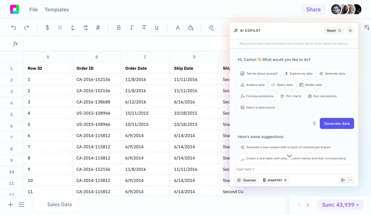
In this guide, we'll define the key components involved in deriving the inverse demand function and provide step-by-step calculations. By the end of this article, you'll have a clear understanding of how to perform these calculations effectively. Furthermore, we'll explore how Sourcetable's AI-powered spreadsheet assistant can streamline this process, offering a user-friendly interface for complex economic calculations. Experience the convenience and enhanced productivity by signing up at app.sourcetable.com/signup.

How to Calculate Inverse Demand Function

Understanding the Basics

The inverse demand function, essential in economics and business calculations, converts a demand function into a price function. This function, critical for determining the price based on quantity demanded, clarifies market dynamics and pricing strategy.

Components Required

Before calculation, ensure you have the demand function, marginal revenue function, and marginal cost function. These components form the basis for deriving the inverse demand, total revenue, and marginal revenue functions.

Calculation Steps

Start with the given demand function (Q = f(P)) and isolate P by rearranging the equation. For example, from Q = 240 - 2P, solve P = 120 - 0.5Q to get the inverse demand function. This equation, now expressing P as a function of Q, serves as the average revenue function.

Utilization in Revenue and Profit Calculations

Use the inverse demand function to calculate total revenue (TR = PQ) and derive marginal revenue (MR), which is the first derivative of total revenue. Businesses apply these calculations to determine optimal production levels, aligning where marginal revenue equals marginal cost for maximum profit.

Practical Example

Consider a demand function for gasoline: Q = 12 - 0.5P. The inverse demand function reverts to P = 24 - 2Q. This setup suggests that price adjusts inverse to changes in quantity, fundamental for pricing strategies in responsive markets.

How to Calculate the Inverse Demand Function

An inverse demand function, crucial for understanding market dynamics, calculates price as a function of quantity demanded. It is instrumental in deriving economic metrics such as average revenue and marginal revenue, and it aids in determining optimal pricing strategies. This guide provides a step-by-step approach to calculating the inverse demand function.

Starting with the Demand Function

Begin with the standard demand function, typically given in the form Q = a - bP, where Q represents the quantity demanded, a is the quantity intercept, and b is the price coefficient. This form indicates how quantity demanded varies with price.

Rearranging the Demand Function

Rearrange this equation to solve for P. This can be achieved by transposing the terms involving P to one side of the equality, making price the subject of the formula. The resultant equation, P = a/b - (1/b)Q, represents the inverse demand function, where a/b signifies the maximum price at zero quantity (intercept) and 1/b reflects the negative slope of the demand curve.

Understanding Economic Implications

The inverse demand function, also known as the price function, aligns price with the quantity demanded. It is identical to the average revenue function, signifying that price also represents the average revenue per unit sold. Additionally, it serves as the foundation for deriving the total revenue (TR) function, given by TR = PQ, and the marginal revenue (MR) function, which is crucial for finding profit-maximizing output levels.

By mastering the calculation of the inverse demand function, businesses and economists can effectively analyze market conditions and set optimal pricing policies, essential for maximizing revenue and profit.

Examples of Calculating the Inverse Demand Function

Example 1: Basic Linear Demand Function

The demand function is given by P = 50 - 2Q. To find its inverse, solve for Q in terms of P. Rearranging, we get Q = 25 - 0.5P. This is the inverse demand function.

Example 2: Including a Constant

Consider a demand function with a constant term: P = 100 - 5Q + 30. Solve for Q to find the inverse. After rearranging, the inverse demand function is Q = 26 - 0.2P.

Example 3: Using a Quadratic Demand Function

For a quadratic demand function P = 120 - 3Q + Q^2, solving for Q gives a more complex form. The inverse demand function, derived from factoring and simplifying, is Q = -1 + \sqrt{1 + 0.25P}.

Example 4: Exponential Demand Function

Given the exponential function P = 80 \exp(-0.05Q), solve for Q. This results in the inverse demand function Q = -20 \ln(0.0125P).

Example 5: Demand Function with Price Elasticity

With the demand function P = 200(0.9)^Q, applying logarithmic properties in rearrangement finds the inverse function: Q = \log_{0.9}\left(\frac{P}{200}ight).

Master Complex Calculations with Sourcetable

Understanding Inverse Demand Function

Grasping the concept of the inverse demand function is crucial for economics students and professionals. This function, denoted as P = f(Q), represents the price P at which consumers are willing to purchase quantity Q of a good. Sourcetable simplifies the learning and application process by providing an intuitive platform to compute and analyze economic models including how to calculate inverse demand function.

AI-Powered Calculations

Sourcetable’s AI-assistant sets it apart, making it an exemplary tool for both education and professional work. It does more than just perform calculations; it explains them. This capability is especially useful when dealing with complex economic formulas and ensures that users not only get results but also understand the computational process.

Efficiency in Learning and Application

Whether you are studying for an exam or need to apply complex theoretical models in the workplace, Sourcetable offers a versatile solution. By inputting your data or equation, you can receive immediate solutions along with explanations, thus speeding up the learning curve and enhancing productivity at work.

Conclusion

Understanding how to calculate the inverse demand function is crucial for economic and business analysis, allowing for precise insights into consumer behavior and pricing strategies. With the mathematical formula P = a/b - Q/b, where P represents price, a is the intercept, b the slope coefficient, and Q the quantity, economic professionals can derive essential market information.

Simplifying Calculations with Sourcetable

Sourcetable, an AI-powered spreadsheet tool, facilitates complex calculations such as the inverse demand function. Its intuitive interface allows users to apply and test calculations on AI-generated data effortlessly, making it an invaluable resource for economists and analysts.

Experience the powerful features of Sourcetable and explore its capabilities by signing up for a free trial at app.sourcetable.com/signup.