Introduction
Understanding how to calculate concentration from absorbance is crucial for professionals working in chemistry and related fields. This calculation is essential for interpreting data from spectrophotometric analyses, which are commonly used to determine the concentration of substances in a solution based on light absorption. The process involves using the Beer-Lambert Law, which relates absorbance to concentration through the absorption coefficient and path length.
To perform this calculation accurately, you need the right tools and knowledge about specific variables such as wavelength and the substance's molar absorptivity. In this guide, we will provide you with a step-by-step approach to calculating concentration from absorbance. Additionally, we will explore how Sourcetable facilitates this process with its AI-powered spreadsheet assistant, enhancing your data analysis capabilities. You can experience these features by signing up at app.sourcetable.com/signup.
See how easy it is to concentration from absorbance with Sourcetable

How to Calculate Concentration from Absorbance
Understanding Beer's Law
Beer's law, expressed as A = mCl, is fundamental when determining the concentration of a solution from absorbance. In this equation, A represents absorbance, m the molar extinction coefficient, C the concentration, and l the path length, typically 1 cm.
Essential Equipment and Materials
To accurately measure absorbance, a UV/Vis spectrophotometer or a photometer is required. Additionally, you'll need a set of standards to create a reliable standard curve, which is crucial for accurate concentration calculations.
Creating a Standard Curve
Start by plotting concentration (x-axis) against absorbance (y-axis) using your standards to form a standard curve. Fit a line of best fit to these data points, ideally in the form y = mx + b, where m is the slope representing the molar extinction coefficient, and b is the y-intercept.
Calculating Concentration
To find the concentration of an unknown sample, use the absorbance value in the line of best fit equation. Solve for concentration C with the formula C = (A - b)/m. Ensure the absorbance and the values for m and b are derived from the same conditions and units to maintain accuracy.
How to Calculate Concentration from Absorbance
Understanding Beer's Law
Beer's Law is central in calculating concentration from absorbance. It is expressed as A = mCl, where A represents absorbance, m is the molar extinction coefficient, C is the concentration, and l is the path length in centimeters. This law indicates that absorbance is directly proportional to concentration, which forms the basis for the calculation.
Creating a Standard Curve
To use Beer's Law effectively, first create a standard curve by plotting known concentrations of a solution against measured absorbance. This is plotted with concentration on the x-axis and absorbance on the y-axis. Applying a line of best fit, usually linear, allows for the determination of the slope (m) and y-intercept (b) of the line.
Calculating Concentration
With the standard curve established, the concentration of an unknown sample can be calculated using the formula C = (A - b) / m. Here, A is the absorbance of the unknown sample, b is the y-intercept from the standard curve, and m is the slope or the molar extinction coefficient derived from the standard curve. This formula rearranges Beer's Law to solve for concentration, C.
Practical Considerations
Ensure accurate measurements of absorbance and correct plotting of the standard curve to reliably use this method. Any error in these initial steps can significantly affect the calculation of concentration, impacting the results' accuracy.
Examples of Calculating Concentration from Absorbance
Example 1: Direct Calculation with Beer's Law
To calculate concentration using Beer's Law, apply the formula C = A / (ε * l). Here, C is the concentration, A is absorbance, ε is the molar absorptivity, and l is the path length of the cuvette. For example, with an absorbance of 0.5, a molar absorptivity of 100 M-1cm-1, and a path length of 1 cm, the concentration is 0.005 M.
Example 2: Using a Standard Curve
First, create a standard curve by measuring the absorbance of known concentrations. Plot these on a graph with concentration on the x-axis and absorbance on the y-axis. To find an unknown concentration, measure the absorbance, then use the graph to find the corresponding concentration. For instance, an absorbance of 0.3 might correlate to a concentration of 0.015 M on the standard curve.
Example 3: Adjusting for Dilution Factor
If a sample was diluted before measurement, calculate the original concentration by multiplying the concentration obtained from Beer's Law or a standard curve by the dilution factor. For example, if the concentration after dilution is 0.01 M and the dilution factor was 5, the original concentration is 0.05 M.
Example 4: Serial Dilutions
Serial dilutions can help when the absorbance is too high or falls outside the standard curve range. Calculate each dilution's concentration, then perform absorbance measurements. Use the final dilution's data to calculate back to the original concentration, accounting for each dilution step. If the final dilution concentration is 0.02 M and it's the third of a series with each dilution reducing concentration by half, the original concentration is 0.16 M.
Example 5: Concentration Ranges
For a broad range of concentrations, it might be practical to prepare multiple samples at different known concentrations. Measure each sample's absorbance, applying Beer's Law to find the best match for your unknown sample’s absorbance. This helps in ensuring measurement accuracy across a wide range.
Discover the Power of Sourcetable for Accurate Calculations
Streamlined Calculation Process
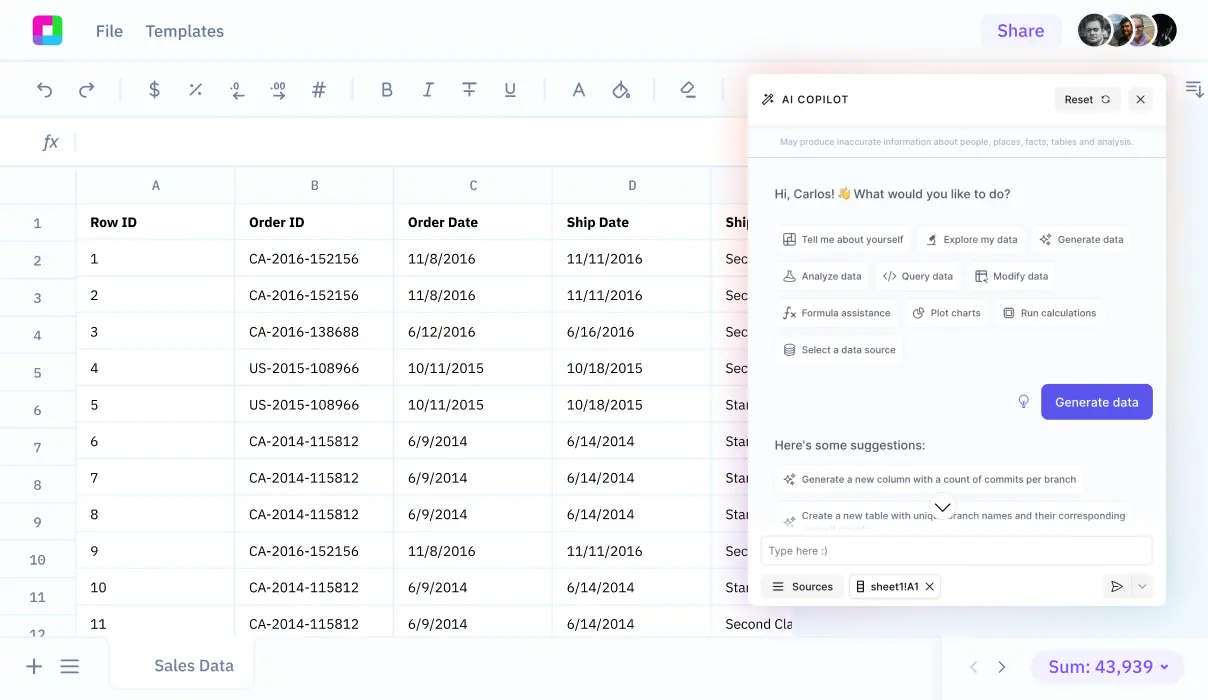
Sourcetable transforms how professionals and students calculate complex formulas by integrating an AI-powered assistant into its spreadsheet environment. Whether you're determining financial projections or solving scientific equations, Sourcetable ensures accuracy and efficiency.
How to Calculate Concentration from Absorbance
For students and researchers wondering how to calculate concentration from absorbance, Sourcetable offers a seamless solution. Simply input your absorbance values, and the AI assistant will utilize the Beer-Lambert Law—A = εlc, where A is absorbance, ε is the molar absorptivity, l is the path length, and c is the concentration—to instantly compute the concentration. Results and complete calculation steps are displayed directly in the spreadsheet, with additional explanations available through the chat interface.
Enhanced Learning and Professional Development
Whether preparing for an exam or conducting professional research, Sourcetable's AI-powered spreadsheets act as both a computational tool and an educational resource. The ability to see both calculations and underlying concepts fosters deeper understanding and retention of knowledge.
Explore the capabilities of Sourcetable to see how it can elevate your calculation proficiency and productivity in educational or professional settings.
Use Cases Unlocked by Knowing How to Calculate Concentration from Absorbance
Medical Diagnostics |
Photometric methods enable quick and cost-effective concentration determinations of various biomarkers in clinical samples, facilitating diagnoses in medical settings. |
Molecular Biology Research |
Researchers can accurately quantify nucleic acids and proteins by measuring absorbance at specific wavelengths—260 nm for nucleic acids and 280 nm for proteins—enhancing precision in molecular analysis. |
Environmental Monitoring |
Concentration calculations from absorbance are vital in assessing pollutant levels in environmental samples, providing data essential for environmental protection and regulatory compliance. |
Pharmaceutical Quality Control |
In pharmaceutical manufacturing, ensuring the correct concentration of active ingredients and excipients through absorbance measurements guarantees product safety and efficacy. |
Food and Beverage Industry |
Using UV/VIS spectroscopy to determine concentrations of food dyes and additives ensures compliance with safety standards and maintains industry quality controls. |
Academic Teaching and Research |
Understanding and applying the principles of UV/VIS spectroscopy in educational institutions bolster hands-on training and experimental design in chemistry and biochemistry courses. |
Industrial Chemical Analysis |
Calculation of chemical concentrations through absorbance readings supports process monitoring and quality assurance in chemical production environments. |
Frequently Asked Questions
How do you calculate concentration from absorbance using Beer's Law?
To calculate concentration from absorbance using Beer's Law, use the equation A = mCl, where A is absorbance, m is the molar extinction coefficient, C is concentration, and l is the path length. Rearrange the equation to solve for C, which yields C = A / (m * l).
What is a standard curve and how is it used to calculate concentration from absorbance?
A standard curve is a graph plotting concentration on the x-axis against absorbance on the y-axis. To create a standard curve, measure the absorbance of known concentrations and plot these data points. Add a line of best fit, typically in the form y = mx + b, where y represents absorbance and x represents concentration. To find the concentration of an unknown sample, find its absorbance on the y-axis, follow it to the line of best fit, and then read off the corresponding concentration value on the x-axis.
What does each component represent in the equation A = mCl used in Beer's Law?
In the equation A = mCl from Beer's Law, 'A' represents the absorbance measured, 'm' is the molar extinction coefficient, 'C' is the concentration of the solution, and 'l' refers to the path length of the cuvette used in the measurement, typically 1 cm.
How do you find concentration if you know the absorbance and the line of best fit equation from a standard curve?
To find the concentration from the line of best fit equation of a standard curve, use the equation C = (A - b)/m, where A is the absorbance, b is the y-intercept, and m is the slope of the line. This equation rearranges the line's equation to solve for concentration (x) when absorbance (y) is known.
Conclusion
Calculating concentration from absorbance is a vital step in various scientific and industrial processes. The formula A = εlc clearly dictates the relationship where A is absorbance, ε is the molar absorptivity, l is the path length, and c is the concentration. Accurate application of this formula ensures precise analytical results and effective product quality management.
Streamline Your Calculations with Sourcetable
Sourcetable, an AI-powered spreadsheet, considerably simplifies this calculation. Its intuitive interface and robust features allow users to seamlessly integrate data, apply formulas, and derive results efficiently. Sourcetable is particularly useful for handling complex datasets and AI-generated data, making it an indispensable tool for researchers and professionals.
Experience the efficiency of Sourcetable by signing up for a free trial today at app.sourcetable.com/signup.
Recommended Guides
Connect your most-used data sources and tools to Sourcetable for seamless analysis.
- how to calculate absorbance from transmittance
- how to calculate molar absorption coefficient
- how to calculate corrected absorbance
- how do you calculate the absorption rate
- how to calculate conc from absorbance
- how to calculate concentration from titration
- how to calculate final concentration
- how to calculate the concentration of a dilute solution

