Introduction
Understanding the long run equilibrium price is vital for businesses and economic analysts aiming to predict market behaviors accurately. This measure indicates the market price at which the quantity supplied equals the quantity demanded, establishing stability without external influences. Essential in both microeconomic models and real-world market analysis, it serves as a cornerstone for pricing strategies and economic forecasting.
In this guide, we delve into the principles and computations involved in determining the long run equilibrium price. We will cover various models and factors influencing this equilibrium, offering you practical insights and computational tools. Particularly, we will explore how Sourcetable enhances this process with its AI-powered spreadsheet assistant, making intricate calculations more accessible. Experience it firsthand at app.sourcetable.com/signup.
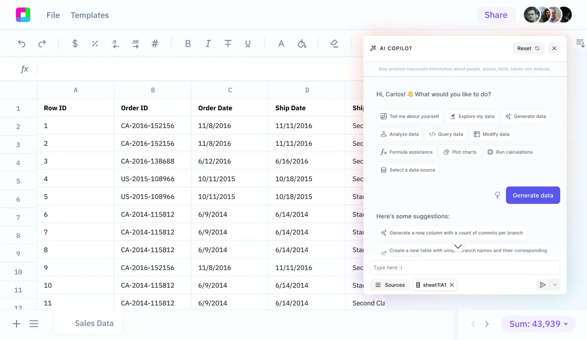
See how easy it is to long run equilibrium price with Sourcetable
How to Calculate Long Run Equilibrium Price
To calculate the long run equilibrium price, adhere to the principles of managerial economics, focusing on the relationship between marginal cost and average total cost. This process ensures businesses can determine the price point at which they achieve zero economic profit, essential for long-term sustainability in competitive markets.
Understanding Key Concepts
First, understand that in long-run equilibrium, the price should equal both the minimum long-run average total cost (LRATC) and the marginal cost (MC). The marginal cost curve should intersect the minimum point of the average total cost curve, indicating the least cost per unit for optimal output levels.
Steps to Calculate Equilibrium Price
To find the long run equilibrium price, follow these steps:1. Identify the Average Total Cost (ATC) formula specific to the firm or scenario.2. Calculate the derivative of the ATC to ascertain the relationship to output (q).3. Set this derivative to zero and solve for q to determine the quantity that minimizes ATC.4. Insert this q value back into the ATC equation to find the minimum ATC, which equals the long run equilibrium price.
For example, if ATC = 12,500/q, take its derivative which results in -12,500/q^2. Setting the derivative to zero and solving for q, you calculate the output level that minimizes ATC. By inputting this quantity into the original ATC formula, the resulting figure represents the long run equilibrium price.
Firms operating under perfect competition, monopolistic competition, or oligopoly must adapt to these calculations to maintain profitability and market share in response to new entrants and competitive pressures.
Correct application of these principles allows firms to navigate their pricing strategy efficiently, maximizing their market position and ensuring adherence to economic profit benchmarks.
How to Calculate Long Run Equilibrium Price
The calculation of the long run equilibrium price is crucial in understanding market dynamics and ensuring sustainable business operations. This price is determined where supply meets demand and is characterized by zero economic profit for firms, meaning no incentives for new entries or exits in the market.
Determining Long Run Equilibrium Price
To find the long run equilibrium price, follow these essential steps:
Identify the average total cost (ATC) and marginal cost (MC) of the firm. The long run equilibrium price occurs at the minimum point of the average total cost curve, where MC = ATC. This is also where marginal cost equals marginal revenue (MC = MR).
Use the derivative of the average total cost function to find this minimum point. Set this derivative equal to zero (d(ATC)/dq = 0) and solve for the quantity (q). This identifies the output level at which the cost is minimized.
Finally, set the long run equilibrium price equal to this minimum average total cost. This ensures that the firm earns zero economic profit, stabilizing the market.
Practical Example
For an average total cost function ATC = 12500/q, take the derivative and set it to zero to find q. Solving this provides a quantity of 500 units, where the ATC is minimized. Therefore, the long run equilibrium price is $60.00 at this level of output, ensuring the firm operates effectively without making economic profits or losses.
This straightforward approach to calculating the long run equilibrium price is vital for businesses to maintain competitiveness and profitability in the long term.
Try Sourcetable For Free
Calculate anything with Sourcetable AI. Tell Sourcetable what you want to calculate. Sourcetable does the rest.
Sign Up
Examples of Calculating Long-Run Equilibrium Price
Example 1: Perfect Competition
In perfect competition, the long-run equilibrium price can be found where the market demand equals market supply. Assume the market demand is represented by P_D = 100 - 10P and the market supply by P_S = 20 + 5P. Setting P_D = P_S gives 100 - 10P = 20 + 5P. Solving for P provides the equilibrium price P = 5.33.
Example 2: Monopolistic Competition
In monopolistic competition, firms have some market power, which affects pricing. To find the long-run equilibrium price, you can use the formula P = ATC, where ATC is average total cost. If ATC = 3 + 0.5Q, and the firm maximizes profit at Q = 10, substitute to find P = 3 + 0.5*10 = 8.
Example 3: Oligopoly
Oligopolies can be more complex due to inter-firm dependence. Using Cournot's duopoly model with firms having symmetric linear cost and demand functions, where total quantity Q = Q_1 + Q_2, and inverse demand function P = a - bQ, equilibrium price can be derived. For firms with identical cost functions c, equilibrium output for each, Q_1 = Q_2 = (a - c)/3b, leads to price P = a - b((a - c)/3b + (a - c)/3b).
Example 4: Utility Function Approach
A utility function approach helps to identify the price that maximizes consumer satisfaction in equilibrium. If a utility function is given by U = 4\sqrt{Q}, where Q is quantity, and P = 20 - 2Q represents the demand, setting the derivative of the utility with respect to quantity equal to price gives the equilibrium terms. Solving dU/dQ = P finds the equilibrium price effectively.
Example 5: Input-Output Model for General Equilibrium
In an economy-wide context, long-run equilibrium prices are influenced by the interaction of multiple industries. Through a Leontief input-output model, where P = (I-A)^{-1}w with I as the identity matrix, A as the technology matrix, and w as the vector of input prices, equilibrium prices for all sectors can be derived, revealing the interconnected impact on prices.
Master Economic Calculations with Sourcetable
Understanding complex economic concepts such as long run equilibrium price can be daunting. Sourcetable, an AI-powered spreadsheet tool, simplifies these calculations. Whether you're a student, educator, or professional, Sourcetable enhances your ability to compute and analyze economic models efficiently.
How Sourcetable Simplifies Economic Calculations
Sourcetable's AI assistant is adept at handling various economic calculations, including the how to calculate long run equilibrium price. By simply inputting your market data, Sourcetable's AI processes the information and computes the long run equilibrium price by balancing supply and demand equations where MC = AR = MR, ensuring market efficiency.
The tool displays results in a user-friendly spreadsheet and provides a detailed explanation via a chat interface of how the calculations were made. This dual approach not only gives you the answers you need but also helps you learn the computational process.
Whether for academic purposes, work assignments, or personal interest, Sourcetable offers an indispensable resource for economic analysis. Its intuitive design, paired with robust AI capabilities, makes it an unrivaled tool for learning and professional development.
Use Cases for Calculating Long Run Equilibrium Price
1. Price Setting in Competitive Markets |
Determining the long run equilibrium price helps firms set prices in a perfectly competitive market by equating price with long-run average total cost, ensuring zero economic profits. This practice stabilizes market competition and optimizes resource distribution. |
2. Output Determination for Maximum Profit |
Calculation of the long run equilibrium price enables a firm to determine the optimal output level q that equates marginal revenue (MR) with marginal cost (MC), maximizing profits and ensuring economic stability. |
3. Market Entry and Exit Decisions |
Understanding long run equilibrium price informs firms when to enter or exit the market based on economic profits. Positive economic profits attract new firms, while persistent losses prompt existing firms to exit, maintaining market balance and efficiency. |
4. Economic Forecasting and Planning |
Businesses use long run equilibrium price calculations for strategic planning and forecasting, enabling better decision-making regarding capacity expansions, budget allocations, and long-term investments. |
5. Regulatory and Policy Making |
Governments and regulatory bodies utilize long run equilibrium price analysis to craft policies that promote fair pricing, prevent monopolistic practices, and enhance consumer welfare. |
6. Academic and Economic Research |
This calculation serves as a fundamental concept in economic theories and models, aiding academic research and practical applications in understanding market dynamics and firm behavior. |
7. Investor Analysis |
In financial markets, investors use long run equilibrium price to evaluate the sustainability of a firm’s profits, guiding investment decisions and portfolio management. |
Frequently Asked Questions
How do you calculate the long run equilibrium price in a perfectly competitive market?
To calculate the long run equilibrium price, set the price equal to the minimum average total cost. Find the quantity of output where average total cost is minimized by taking the derivative of the average total cost function, setting it to zero, and solving for the quantity (q). Then, use this quantity to find the price that equals the average total cost.
What conditions must be met for a firm to be in long run equilibrium?
A firm is in long run equilibrium when its price equals its average total cost at the minimum point on its average total cost curve, where marginal cost must also pass through. This condition ensures the firm earns zero economic profit, meaning there is no incentive for new firms to enter or existing firms to exit the market.
Why is the long run equilibrium price considered stable?
The long run equilibrium price is considered stable because it is the price at which firms earn zero economic profit, thus creating no incentive for new firms to enter or existing firms to leave the market. This price stability occurs when firms produce at the lowest possible average total cost.
How does increased competition affect the long run equilibrium price in a market?
In perfectly competitive markets, increased competition due to firms earning higher profits leads to more production, shifting the supply curve to the right. This increases the market supply, which reduces the equilibrium price to a new lower level where firms again earn zero economic profits.
What impacts does the entry of new firms have on the existing firms in a monopolistically competitive market?
In monopolistically competitive markets, the entry of new firms reduces the demand for existing firms, leading to a need for these firms to spend more on advertising and differentiation strategies to maintain their market share and profitability.
Conclusion
Understanding how to calculate the long-run equilibrium price is essential for economics and business strategy. It involves determining the price point at which supply equals demand, ensuring no economic profit is made and market forces are balanced.
Simplifying Calculations with Sourcetable
Using Sourcetable, an AI-powered spreadsheet, simplifies these calculations significantly. It enables users to input data seamlessly and perform complex calculations with ease. Sourcetable's intuitive design and powerful AI tools make it an ideal solution for anyone looking to calculate long-run equilibrium prices efficiently.
Practice with AI-Generated Data
Furthermore, Sourcetable offers the unique feature of allowing users to try their calculations on AI-generated data. This is particularly useful for simulation and training purposes, providing users with practical experience and enhancing their understanding of dynamic market concepts.
Experience the power of Sourcetable's AI-driven calculations and more by signing up for a free trial at app.sourcetable.com/signup.
Try Sourcetable For Free
Calculate anything with Sourcetable AI. Tell Sourcetable what you want to calculate. Sourcetable does the rest.
Sign Up
Recommended Guides
Connect your most-used data sources and tools to Sourcetable for seamless analysis.
Calculate anything you want with AI
Sourcetable takes the math out of any complex calculation. Tell Sourcetable what you want to calculate. Sourcetable AI does the rest. See the step-by-step result in a spreadsheet and visualize your work. No Excel skills required.